Estimate point process parameters using log-likelihood maximization

Estimate spatio-temporal point process parameters by maximizing the (approximate) full log-likelihood using nloptr. For the self-correcting process, the arrival times must be on \((0,1)\) and can either be supplied directly in data as time, or constructed from size via the gentle-decay (power-law) mapping power_law_mapping using delta (single fit) or delta_values (delta search).

Usage

estimate_process_parameters(
  data,
  process = c("self_correcting"),
  x_grid = NULL,
  y_grid = NULL,
  t_grid = NULL,
  upper_bounds = NULL,
  parameter_inits = NULL,
  delta = NULL,
  delta_values = NULL,
  parallel = FALSE,
  num_cores = max(1L, parallel::detectCores() - 1L),
  set_future_plan = FALSE,
  strategy = c("local", "global_local", "multires_global_local"),
  grid_levels = NULL,
  refine_best_delta = TRUE,
  global_algorithm = "NLOPT_GN_CRS2_LM",
  local_algorithm = "NLOPT_LN_BOBYQA",
  global_options = list(maxeval = 150),
  local_options = list(maxeval = 300, xtol_rel = 1e-05, maxtime = NULL),
  n_starts = 1L,
  jitter_sd = 0.35,
  seed = 1L,
  finite_bounds = NULL,
  verbose = TRUE
)

Arguments

data: a data.frame or matrix. Must contain either columns (time, x, y) or (x, y, size). If a matrix is provided for delta search, it must have column names c("x","y","size").
process: character string specifying the process model. Currently supports "self_correcting".
x_grid, y_grid, t_grid: numeric vectors defining the integration grid for \((x,y,t)\).
upper_bounds: numeric vector of length 3 giving c(b_t, b_x, b_y).
parameter_inits: numeric vector of length 8 giving initialization values for the model parameters.
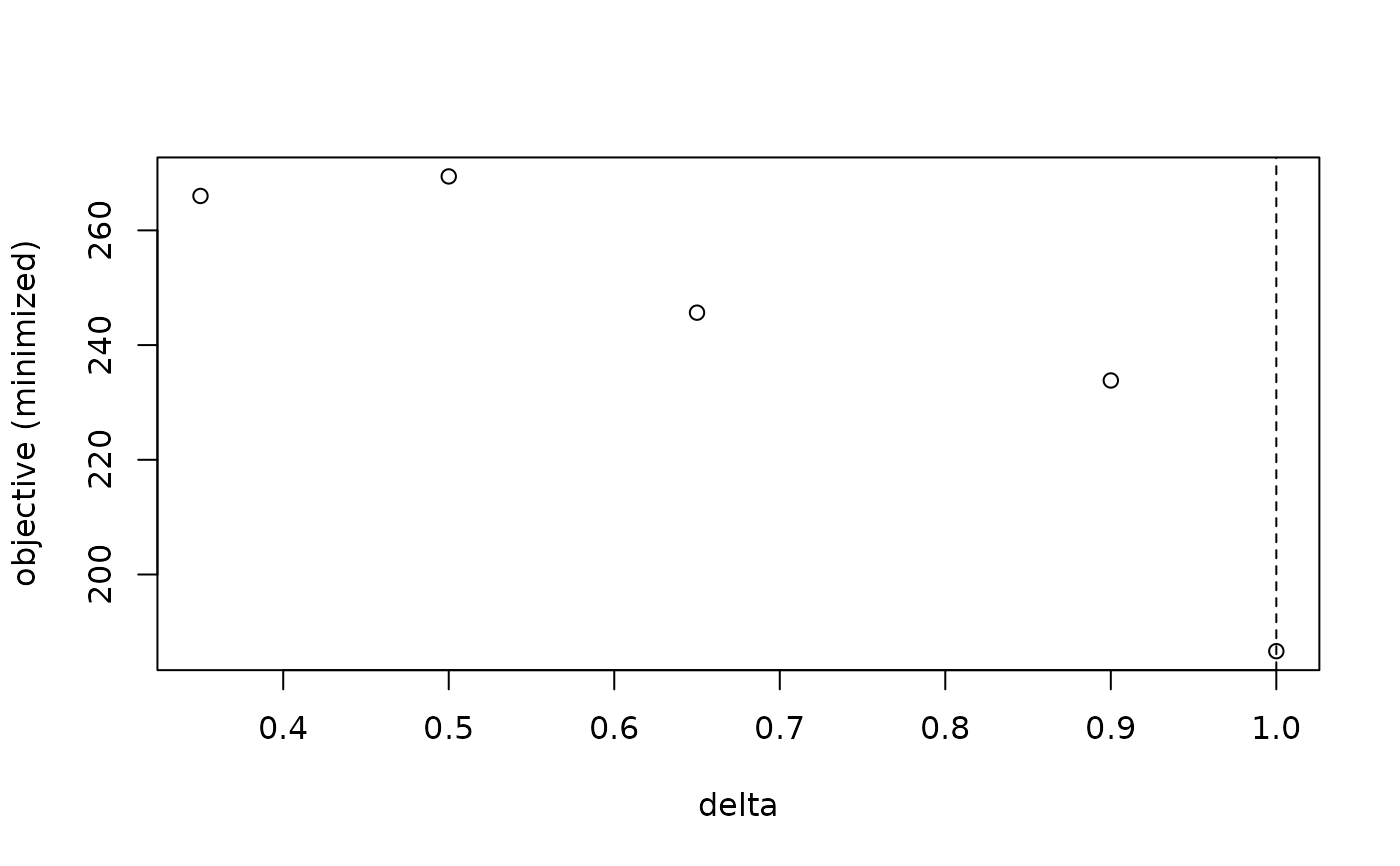
delta: (optional) numeric scalar used only when data contains (x,y,size) but not time.
delta_values: (optional) numeric vector. If supplied, the function fits the model for each value of delta_values (mapping size -> time via power_law_mapping) and returns the best fit (lowest objective).
parallel: logical. If TRUE, uses furrr/future to parallelize either (a) over delta_values (when provided) or (b) over multi-start initializations (when delta_values is NULL and n_starts > 1).
num_cores: Integer number of workers to use when set_future_plan = TRUE.
set_future_plan: TRUE or FALSE, if TRUE, temporarily sets future::plan(multisession, workers = num_cores) and restores the original plan on exit.
strategy: Character string specifying the estimation strategy: - "local": single-level local optimization from parameter_inits. - "global_local": single-level global optimization (from parameter_inits) followed by local polish. - "multires_global_local": multi-resolution fitting over grid_levels (coarsest level uses global + local; finer levels use local polish only).
grid_levels: (optional) list defining the multi-resolution grid schedule when strategy = "multires_global_local". Each entry can be a numeric vector c(nx, ny, nt) or a list with named entries list(nx=..., ny=..., nt=...). If NULL, uses the supplied (x_grid, y_grid, t_grid) as a single level.
refine_best_delta: TRUE or FALSE, if TRUE and delta_values is supplied, performs a final refinement fit at the best delta found using the full multi-resolution strategy.
global_algorithm, local_algorithm: character strings specifying the NLopt algorithms to use for the global and local optimization stages, respectively.
global_options, local_options: named lists of options to pass to nloptr::nloptr() for the global and local optimization stages, respectively.
n_starts: integer number of multi-start initializations to use for the local optimization stage.
jitter_sd: numeric standard deviation used to jitter the multi-start initializations.
seed: integer random seed used for multi-start initialization jittering.
finite_bounds: (optional) list with components lb and ub giving finite lower and upper bounds for all 8 parameters. Used only when the selected optimization algorithms require finite bounds.
verbose: TRUE or FALSE, if TRUE, prints progress messages during fitting.

Value

an object of class "ldmppr_fit" containing the best nloptr fit and (optionally) all fits from a delta search.

Details

For the self-correcting process, the log-likelihood integral is approximated using the supplied grid (x_grid, y_grid, t_grid) over the bounded domain upper_bounds. When delta_values is supplied, this function performs a grid search over delta values, fitting the model separately for each mapped dataset and selecting the best objective value.

References

Møller, J., Ghorbani, M., & Rubak, E. (2016). Mechanistic spatio-temporal point process models for marked point processes, with a view to forest stand data. Biometrics, 72(3), 687–696. doi:10.1111/biom.12466 .

Examples

data(small_example_data)

x_grid <- seq(0, 25, length.out = 5)
y_grid <- seq(0, 25, length.out = 5)
t_grid <- seq(0, 1,  length.out = 5)

parameter_inits <- c(1.5, 8.5, .015, 1.5, 3.2, .75, 3, .08)
upper_bounds <- c(1, 25, 25)

fit <- estimate_process_parameters(
  data = small_example_data,
  process = "self_correcting",
  x_grid = x_grid,
  y_grid = y_grid,
  t_grid = t_grid,
  upper_bounds = upper_bounds,
  parameter_inits = parameter_inits,
  delta = 1,
  strategy = "global_local",
  global_algorithm = "NLOPT_GN_CRS2_LM",
  local_algorithm = "NLOPT_LN_BOBYQA",
  global_options = list(maxeval = 150),
  local_options = list(maxeval = 25, xtol_rel = 1e-2),
  verbose = TRUE
)
#> iteration: 1
#> 	f(x) = 404.701347
#> iteration: 2
#> 	f(x) = 45923038155926103673291145216000.000000
#> iteration: 3
#> 	f(x) = 78087.881491
#> iteration: 4
#> 	f(x) = 171968.209533
#> iteration: 5
#> 	f(x) = 940760247304106907466985088483328.000000
#> iteration: 6
#> 	f(x) = 20017012287594692.000000
#> iteration: 7
#> 	f(x) = 254775.568361
#> iteration: 8
#> 	f(x) = 174158343736330902177636877864870488008832579534848.000000
#> iteration: 9
#> 	f(x) = 201218.394367
#> iteration: 10
#> 	f(x) = 32381.148017
#> iteration: 11
#> 	f(x) = 15058294657.892656
#> iteration: 12
#> 	f(x) = 107943864513997882050839200077666245943009026290043801921106944066584576.000000
#> iteration: 13
#> 	f(x) = 147097287123348780304402743296.000000
#> iteration: 14
#> 	f(x) = 14375379367243273994240.000000
#> iteration: 15
#> 	f(x) = 30070153044072322507472896.000000
#> iteration: 16
#> 	f(x) = 217314.615778
#> iteration: 17
#> 	f(x) = 38670.744812
#> iteration: 18
#> 	f(x) = 1010802732162535189251096576.000000
#> iteration: 19
#> 	f(x) = 106485702101798596202388801556010936441860259840.000000
#> iteration: 20
#> 	f(x) = 66873985828083630638538166783515688281504570915227659403264.000000
#> iteration: 21
#> 	f(x) = 7901633076114307311206400.000000
#> iteration: 22
#> 	f(x) = 91276717821269456.000000
#> iteration: 23
#> 	f(x) = 1148645666142653.500000
#> iteration: 24
#> 	f(x) = 653954833.232074
#> iteration: 25
#> 	f(x) = 22159601.644635
#> iteration: 26
#> 	f(x) = 17233067599545188389627336065024.000000
#> iteration: 27
#> 	f(x) = 101104.434107
#> iteration: 28
#> 	f(x) = 121085.305693
#> iteration: 29
#> 	f(x) = 505474482997232622632359031734028907702051198694935679262855547322368.000000
#> iteration: 30
#> 	f(x) = 8971405842.576874
#> iteration: 31
#> 	f(x) = 111782973114252148736.000000
#> iteration: 32
#> 	f(x) = 844306549745744655417344.000000
#> iteration: 33
#> 	f(x) = 3906492369088589919005543871746037674881843200.000000
#> iteration: 34
#> 	f(x) = 198091.764497
#> iteration: 35
#> 	f(x) = 104662927010373686871656215443598797382523889385472.000000
#> iteration: 36
#> 	f(x) = 230785.686246
#> iteration: 37
#> 	f(x) = 153600543133855134955337390897630289781063680.000000
#> iteration: 38
#> 	f(x) = 165386943553418657792.000000
#> iteration: 39
#> 	f(x) = 294412.973215
#> iteration: 40
#> 	f(x) = 385051795701.325012
#> iteration: 41
#> 	f(x) = 96398601805121156284416.000000
#> iteration: 42
#> 	f(x) = 164366153952334025844246376885068721851523206745172374314946502544326656.000000
#> iteration: 43
#> 	f(x) = 12453106510695707443200.000000
#> iteration: 44
#> 	f(x) = 246192.058728
#> iteration: 45
#> 	f(x) = 20415725700646879424141066240.000000
#> iteration: 46
#> 	f(x) = 338634619072566.000000
#> iteration: 47
#> 	f(x) = 68195845750752668549120.000000
#> iteration: 48
#> 	f(x) = 105156637364695.687500
#> iteration: 49
#> 	f(x) = 4440816766978062163988447232.000000
#> iteration: 50
#> 	f(x) = 2786416611.047494
#> iteration: 51
#> 	f(x) = 156592725560245249369964544.000000
#> iteration: 52
#> 	f(x) = 212718543402225078931455252723370332179315439735785601570497888256.000000
#> iteration: 53
#> 	f(x) = 747590996447196.000000
#> iteration: 54
#> 	f(x) = 7558982430442756253941760.000000
#> iteration: 55
#> 	f(x) = 30827315293811611009024.000000
#> iteration: 56
#> 	f(x) = 150671.915023
#> iteration: 57
#> 	f(x) = 896721095489466594936726878372992385024.000000
#> iteration: 58
#> 	f(x) = 139223.217097
#> iteration: 59
#> 	f(x) = 133907.064272
#> iteration: 60
#> 	f(x) = 40340.465061
#> iteration: 61
#> 	f(x) = 7222956718646460538886673316725481537536.000000
#> iteration: 62
#> 	f(x) = 906106223317.164429
#> iteration: 63
#> 	f(x) = 216375.348560
#> iteration: 64
#> 	f(x) = 2737546883.053558
#> iteration: 65
#> 	f(x) = 364714488112.936584
#> iteration: 66
#> 	f(x) = 138188207947423888.000000
#> iteration: 67
#> 	f(x) = 662161381610068470437680272086747842609152.000000
#> iteration: 68
#> 	f(x) = 164156.770154
#> iteration: 69
#> 	f(x) = 1993493441896515214502321975197696.000000
#> iteration: 70
#> 	f(x) = 43071126334185040820097154700736987136.000000
#> iteration: 71
#> 	f(x) = 12694315964512.470703
#> iteration: 72
#> 	f(x) = 46292227.462435
#> iteration: 73
#> 	f(x) = 597869393769638474905800032085960082401027095379407347384320.000000
#> iteration: 74
#> 	f(x) = 251719908430498799362378360671054313029632.000000
#> iteration: 75
#> 	f(x) = 30775311642453508096.000000
#> iteration: 76
#> 	f(x) = 70004.959765
#> iteration: 77
#> 	f(x) = 48895.313312
#> iteration: 78
#> 	f(x) = 26096.067108
#> iteration: 79
#> 	f(x) = 7857261346491830563426363724791808.000000
#> iteration: 80
#> 	f(x) = 41823574117923445222716473344.000000
#> iteration: 81
#> 	f(x) = 183845723254411111694336.000000
#> iteration: 82
#> 	f(x) = 483066781178.234009
#> iteration: 83
#> 	f(x) = 261093.910842
#> iteration: 84
#> 	f(x) = 283941229676853752965890048.000000
#> iteration: 85
#> 	f(x) = 87752.130227
#> iteration: 86
#> 	f(x) = 231107273213.754242
#> iteration: 87
#> 	f(x) = 376101071705449363985628397568.000000
#> iteration: 88
#> 	f(x) = 1546403401225115034276618970244253807558336348065628160.000000
#> iteration: 89
#> 	f(x) = 7657006205025329110148308660838727680.000000
#> iteration: 90
#> 	f(x) = 667883231646187.750000
#> iteration: 91
#> 	f(x) = 8752.895823
#> iteration: 92
#> 	f(x) = 45113857.979421
#> iteration: 93
#> 	f(x) = 3317473876001.270996
#> iteration: 94
#> 	f(x) = 9907056567260950.000000
#> iteration: 95
#> 	f(x) = 3664195.141817
#> iteration: 96
#> 	f(x) = 745074920119510214581600387072.000000
#> iteration: 97
#> 	f(x) = 136137856620.304489
#> iteration: 98
#> 	f(x) = 155843.002185
#> iteration: 99
#> 	f(x) = 38953514741537432832776050370130626851922274942976.000000
#> iteration: 100
#> 	f(x) = 6269666523972620.000000
#> iteration: 101
#> 	f(x) = 1497408810818644424211429335236608.000000
#> iteration: 102
#> 	f(x) = 193013901141598371840.000000
#> iteration: 103
#> 	f(x) = 817182132595478370037755147201513209419071621051965900387778560.000000
#> iteration: 104
#> 	f(x) = 1842.843150
#> iteration: 105
#> 	f(x) = 471614.091710
#> iteration: 106
#> 	f(x) = 2002070293371325959558785505689600.000000
#> iteration: 107
#> 	f(x) = 384710.887866
#> iteration: 108
#> 	f(x) = 222467030067.887329
#> iteration: 109
#> 	f(x) = 22397.213129
#> iteration: 110
#> 	f(x) = 39174.045770
#> iteration: 111
#> 	f(x) = 421940.452065
#> iteration: 112
#> 	f(x) = 105170.071978
#> iteration: 113
#> 	f(x) = 5787967828003260416.000000
#> iteration: 114
#> 	f(x) = 107340.265310
#> iteration: 115
#> 	f(x) = 3650695277460.000000
#> iteration: 116
#> 	f(x) = 5112385967418802933990404208972891527315672870521703820954756448256.000000
#> iteration: 117
#> 	f(x) = 717.538863
#> iteration: 118
#> 	f(x) = 3236014711056652208495750139786395524268032.000000
#> iteration: 119
#> 	f(x) = 1431264.751184
#> iteration: 120
#> 	f(x) = 11401.650042
#> iteration: 121
#> 	f(x) = 9145.616576
#> iteration: 122
#> 	f(x) = 9862037240323361371899185035422104985131810816.000000
#> iteration: 123
#> 	f(x) = 1583.942957
#> iteration: 124
#> 	f(x) = 115325.466740
#> iteration: 125
#> 	f(x) = 6954177.308699
#> iteration: 126
#> 	f(x) = 35549.611541
#> iteration: 127
#> 	f(x) = 2192225649838467472949248.000000
#> iteration: 128
#> 	f(x) = 2279822572316647.000000
#> iteration: 129
#> 	f(x) = 175645.762059
#> iteration: 130
#> 	f(x) = 355386.797053
#> iteration: 131
#> 	f(x) = 25173413066597.238281
#> iteration: 132
#> 	f(x) = 26238250738.606255
#> iteration: 133
#> 	f(x) = 26659.672197
#> iteration: 134
#> 	f(x) = 8022157.458195
#> iteration: 135
#> 	f(x) = 13194.682213
#> iteration: 136
#> 	f(x) = 9315662265147977555921960956067193682691055785380256153600.000000
#> iteration: 137
#> 	f(x) = 2100.416559
#> iteration: 138
#> 	f(x) = 7342883254405956.000000
#> iteration: 139
#> 	f(x) = 452957.242745
#> iteration: 140
#> 	f(x) = 35821471315227391629186826240.000000
#> iteration: 141
#> 	f(x) = 39030.316192
#> iteration: 142
#> 	f(x) = 334505352333192.687500
#> iteration: 143
#> 	f(x) = 326655279841829.812500
#> iteration: 144
#> 	f(x) = 12732536935000506.000000
#> iteration: 145
#> 	f(x) = 2264257.790699
#> iteration: 146
#> 	f(x) = 2305065.194891
#> iteration: 147
#> 	f(x) = 28798.220003
#> iteration: 148
#> 	f(x) = 63662.306827
#> iteration: 149
#> 	f(x) = 647253809085.549805
#> iteration: 150
#> 	f(x) = 111802587299600351232.000000

coef(fit)
#> [1] 1.5000000 7.6837649 0.0302285 1.5000000 3.2000000 0.7500000 3.0000000
#> [8] 0.0800000
logLik(fit)
#> 'log Lik.' -269.0724 (df=8)

# \donttest{
# Delta-search example (data has x,y,size; time is derived internally for each delta)
fit_delta <- estimate_process_parameters(
  data = small_example_data, # x,y,size
  process = "self_correcting",
  x_grid = x_grid,
  y_grid = y_grid,
  t_grid = t_grid,
  upper_bounds = upper_bounds,
  parameter_inits = parameter_inits,
  delta_values = c(0.35, 0.5, 0.65, 0.9, 1.0),
  parallel = TRUE,
  set_future_plan = TRUE,
  num_cores = 2,
  strategy = "multires_global_local",
  grid_levels = list(
  list(nx = 5, ny = 5, nt = 5),
  list(nx = 8, ny = 8, nt = 8),
  list(nx = 10, ny = 10, nt = 10)
  ),
  global_options = list(maxeval = 100),
  local_options  = list(maxeval = 100, xtol_rel = 1e-3),
  n_starts = 3,
  refine_best_delta = TRUE,
  verbose = TRUE
)
#> future plan set to multisession with workers = 2
#> Starting delta search with 5 delta values.
#> Coarse delta search complete. Best delta = 1 (objective=186.63324).
#> Refining best delta across finer grids...
#> Refinement complete (best delta = 1).
plot(fit_delta)

# }